Semi-Discrete Form#
강좌: 기초 전산유체역학
Semi-discrete Formulation#
앞선 수치 기법들은 시간에 대해서 1차 정확도 Euler Explicit 기법을 적용하였다.
공간에 대해서만 차분식을 적용하는 경우 편미분 차분식은 상미분 방정식 해석으로 생각할 수 있다.
공간에 대해 Central 기법을 적용하면 다음과 같다.
이를 각 격자점에 대해 풀어서 표현하면
즉 초기치 상미분 방정식 \(y'=f(y,t), ~y(0)=y^0\) 형태로 생각할 수 있다.
몇 가지 상미분 방정식 해석 방법을 적용해보자.
Revisit Explicit Euler Method#
Euler Explicit Method는 다음과 같다.
정확도#
수치해석시 오차는 다음과 같다.
Trunaction Error
Round-off Error
Local truncation error (LTE)
Euler 기법의 경우 매 시간마다 오차가 발생한다.
LTE가 누적되어 Global truncation error가 된다.
Taylor Expansion 적용하면
\[ y_{n+1} = y_n + h \frac{dy}{dt} + \frac{h^2}{2!} \frac{d^2y}{dt^2} + O(h^3) \]즉 오차는 다음과 같다.
\[ E_t = \frac{h^2}{2!} \frac{d^2y}{dt^2} + O(h^3) = O(h^2). \]전 시간 영역에 대해서 오차가 누적되므로 1차 정확도 (\(O(h)\))가 된다.
Stability of ODE#
안정성을 분석하기 위해 Model problem을 생각한다.
\(\lambda_R < 0\) 인 경우 이 미분방정식은 해가 제한되어 (bounded) 있다.
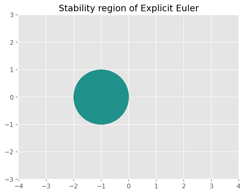
Explicit Euler에 적용하면 다음과 같다.
여기서 \(h=\Delta t\) 이다. 정리하면
여기서 \(|\sigma| < 1\) 일 때 수치 기법의 해가 발산하지 않는다.
%matplotlib inline
from matplotlib import pyplot as plt

import numpy as np

plt.style.use('ggplot')
plt.rcParams['figure.dpi'] = 150
# Make grid
x = np.linspace(-3, 3, 201)
y = np.linspace(-3, 3, 201)
X, Y = np.meshgrid(x, y)
z = X + Y*1j

# Amplication factor of Explicit Euler (z=lambda h)
sig = 1 + z

# Same scale of x and y
plt.axis('equal')

# Stability region
plt.contourf(X,Y,abs(sig), levels=[0, 1])

# Title
plt.title('Stability region of Explicit Euler')
Text(0.5, 1.0, 'Stability region of Explicit Euler')
Matrix Stability#
상미분 방정식의 안정성 개념을 편미분 방정식으로 확장하면, 앞선 연산 행렬의 고유치의 최대 값을 모델 방정식의 \(\lambda\) 로 생각하고 분석할 수 있다.
위 연산 행렬의 고유치는 다음과 같이 알려져 있다.
Explicit Euler 기법의 안정성 영역을 보면 imaginary 축에서는 아주 작은 시간 간격에도 안정하지 않다. 즉 Central Method 가 안정하지 않음을 알 수 있다.
이렇게 안정성을 분석하는 방법을 Matrix stability 라 한다. 다만 연산 행렬의 고유치를 구하는 과정이 쉽지 않다는 단점이 있다.
Modified Wavenumber Analysis#
Von Neumann Stability 방법은 Fully-discrete formulation (time and space)에만 적용할 수 있다.
매우 비슷한 접근법이지만 Semi-discrete formulation에 사용 가능한 방법이 Modified Wavenumber 분석법이다. 이 방법 역시 선형 방정식이고, 경계 조건이 Periodic 일 때 사용 가능하다.
우선 PDE Solution을 \(u(x, t) = \psi(t) e^{ikx}\) 로 생각한다. 이를 Wave 방정식에 적용하면 다음과 같다.
차분식에 이와 같은 Solution \(u_j = \psi(t) e^{ikx_j}\)을 적용했을 때 Wavenumber 가 아래와 같이 변한다.
여기서 \(k'\) 를 Modified Wavenumber 이다.
Central 기법 차분식에 대해 적용해보자.
위 해를 적용하면,
이를 정리하면
차분식에 의해 Modified wavenumber \(k'\) 은 다음과 같다.
Stability 분석을 위해 모델 방정식 형태로 표현하면 \(\lambda = -i a k' \) 이다. 허수이므로 Euler Explicit 에서는 불안정하다.
더 정확한 Explicit Method#
정확도를 높이기 위해서 2가지 방법이 고려된다.
Multi-stage method
한 시간 간격 (step) 을 전진하기 위해 여러 Stage를 계산함
Multi-step method
한 시간 간격을 전진하기 위해 이전 여러 step의 결과를 활용함
이들은 모두 Taylor expansion에서 고차항을 근사한다.
Runge Kutta Method#
Multi-stage 기법에 대표적인 방법으로 다음과 같은 과정으로 계산한다.
Runge Kutta 기법의 계수는 다음 Butcher tableau로 표기한다.
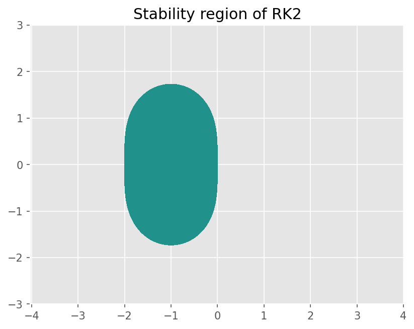
2차 정확도 Runge Kutta Method#
무수히 많은 2차 Runge Kutta 법이 있다.
\[\begin{split} b_1 = 1 -b_2 \\ c_2 = a_{21} = \frac{1}{2 b_2} \end{split}\]이 기법은 2차 정확도를 갖는다.
Huen’s method
\[\begin{split} \begin{array}{c|cc} 0 & 0 & \\ 1 & 1 & 0 \\ \hline & 1/2 & 1/2 \end{array} \end{split}\]Midpoint method
\[\begin{split} \begin{array}{c|cc} 0 & 0 & \\ 1/2 & 1/2 & 0 \\ \hline & 0 & 1 \end{array} \end{split}\]
이 기법의 Stability는 다음과 같다.
4차 정확도 Runge Kutta Method#
이 기법은 4차 정확도를 갖는다.
이 기법의 Stability는 다음과 같다.
# Make grid
xx = np.linspace(-3, 3, 201)
yy = np.linspace(-3, 3, 201)
X, Y = np.meshgrid(xx, yy)
z = X + Y*1j

# Amplication factor of Explicit Euler (z=lambda h)
sig = 1 + z + 0.5*z**2

# Same scale of x and y
plt.axis('equal')

# Stability region
plt.contourf(X,Y,abs(sig), levels=[0, 1])

# Title
plt.title('Stability region of RK2')
Text(0.5, 1.0, 'Stability region of RK2')
# Make grid
xx = np.linspace(-3, 3, 201)
yy = np.linspace(-3, 3, 201)
X, Y = np.meshgrid(xx, yy)
z = X + Y*1j

# Amplication factor of RK4 (z=lambda h)
sig = 1 + z + 0.5*z**2 + z**3/6 + z**4/24

# Same scale of x and y
plt.axis('equal')

# Stability region
plt.contourf(X,Y,abs(sig), levels=[0, 1])

# Title
plt.title('Stability region of RK4')
Text(0.5, 1.0, 'Stability region of RK4')
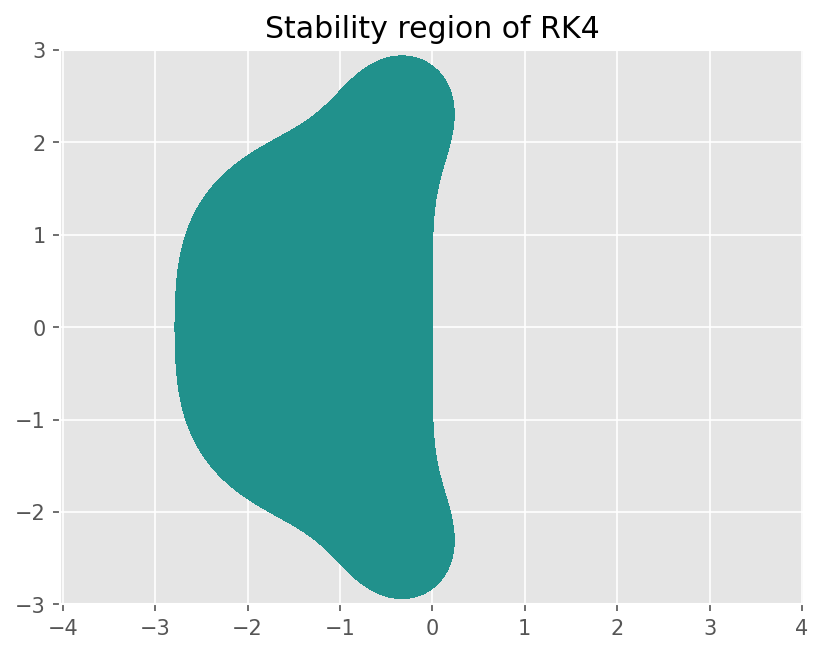
4차 Runge Kutta 기법을 안정성 영역은 \(\lambda h\) 가 imaginary 축에서도 2.83까지 안정하다. 이를 적용한 Central difference 기법에 대해 경우 Modified wavenumber Analysis 결과는 다음과 같다.
즉
예제#
Modified Wavenumber analysis#
Upwind 기법에 대한 Modified wavenumber 분석을 Real axis에서 수행하고, Euler Explicit 및 4차 Runge Kutta 기법을 적용했을 때 안정성을 분석하시오.
수치 실험#
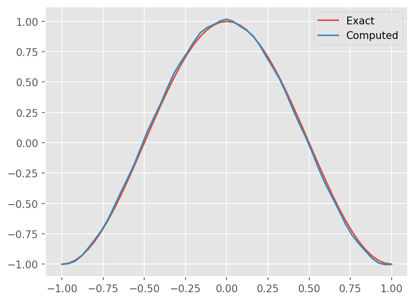
공간에 대해 Central, Upwind 차분법을 적용하고 시간에 대해서 4차 Runge Kutta 기법을 적용하자. Sine wave 문제를 해석해보자.
계산 시간을 늘려보자 (\(t=5, 10, 15, 20\))
시간 간격을 늘려보고, Stability 결과와 비교해보자.
def central_rhs(nx, u, dx, a, du):
    for i in range(1, nx+2):
        du[i] = -0.5*a*(u[i+1] - u[i-1])/dx
def bc_periodic(u):
    # index (nx : -3), (nx+2 : -1)
    u[0] = u[-3]
    u[-1] = u[2]
a = 1.0

nx = 50
cfl = 0.9
t_target = 15.5

# Make grid
x = np.linspace(-1, 1, nx+1)
dx = np.diff(x)[0]

# Solution array
u = np.empty(nx+3)
u0 = np.empty_like(u)
k1 = np.zeros_like(u)
k2 = np.zeros_like(u)

# Initialize
u[1:-1] = np.sin(np.pi*x)
bc_periodic(u)

# Time step
dt = cfl*dx/a

# Calculation
t = 0
while abs(t - t_target) > 1e-8:
    # Adjust time step to reach target time
    dt = min(dt, t_target - t)

    # First stage
    u0[:] = u
    bc_periodic(u)
    central_rhs(nx, u, dx, a, k1)
    u += 0.5*dt*k1

    # Second stage
    bc_periodic(u)
    central_rhs(nx, u, dx, a, k2)
    u = u0 + dt*k2

    # Update
    t += dt

# Exact solution
u_exact = np.sin(np.pi*(x-a*t))
plt.plot(x, u_exact)
plt.plot(x, u[1:-1])
plt.legend(['Exact', 'Computed'])
<matplotlib.legend.Legend at 0x7fea88b36950>